Constant elasticity of variance model

In mathematical finance, the CEV or constant elasticity of variance model is a stochastic volatility model, although technically it would be classed more precisely as a local volatility model, that attempts to capture stochastic volatility and the leverage effect. The model is widely used by practitioners in the financial industry, especially for modelling equities and commodities. It was developed by John Cox in 1975.

Dynamic

The CEV model is a stochastic process which evolves according to the following stochastic differential equation:

${\displaystyle \mathrm {d} S_{t}=\mu S_{t}\mathrm {d} t \sigma S_{t}^{\gamma }\mathrm {d} W_{t}}$

in which S is the spot price, t is time, and μ is a parameter characterising the drift, σ and γ are volatility parameters, and W is a Brownian motion. It is a special case of a general local volatility model, written as

${\displaystyle \mathrm {d} S_{t}=\mu S_{t}\mathrm {d} t v(t,S_{t})S_{t}\mathrm {d} W_{t}}$

where the price return volatility is

${\displaystyle v(t,S_{t})=\sigma S_{t}^{\gamma -1}}$

The constant parameters ${\displaystyle \sigma ,\;\gamma }$ satisfy the conditions ${\displaystyle \sigma \geq 0,\;\gamma \geq 0}$.

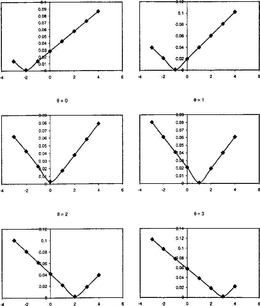
The parameter ${\displaystyle \gamma }$ controls the relationship between volatility and price, and is the central feature of the model. When ${\displaystyle \gamma <1}$ we see an effect, commonly observed in equity markets, where the volatility of a stock increases as its price falls and the leverage ratio increases. Conversely, in commodity markets, we often observe ${\displaystyle \gamma >1}$, whereby the volatility of the price of a commodity tends to increase as its price increases and leverage ratio decreases. If we observe ${\displaystyle \gamma =1}$ this model becomes a geometric Brownian motion as in the Black-Scholes model, whereas if ${\displaystyle \gamma =0}$ and either ${\displaystyle \mu =0}$ or the drift ${\displaystyle \mu S}$ is replaced by ${\displaystyle \mu }$, this model becomes an arithmetic Brownian motion, the model which was proposed by Louis Bachelier in his PhD Thesis "The Theory of Speculation", known as Bachelier model.

See also

• Volatility (finance)
• Stochastic volatility
• Local volatility
• SABR volatility model
• CKLS process

References

External links

• Asymptotic Approximations to CEV and SABR Models
• Price and implied volatility under CEV model with closed formulas, Monte-Carlo and Finite Difference Method
• Price and implied volatility of European options in CEV Model delamotte-b.fr